Building Factor Models on India Stack Data: UPI, AA, and GST as Alpha Signals
India's digital public infrastructure generates signals that don't exist anywhere else. Here's how to turn UPI velocity, Account Aggregator flows, and GST patterns into systematic factors.
India has accidentally built the world’s best alternative data infrastructure for equity factor investing. Not deliberately – nobody at NPCI or GSTN was thinking about systematic trading strategies when they designed these systems. But the result is a set of high-frequency, broad-coverage economic signals that simply do not exist in any other major market.
I have spent the last two years exploring whether these signals can be turned into tradable equity factors. What follows is the methodology, the code, and the results – including where the data falls short and where I wasted time chasing signals that turned out to be noise.
The India Stack Data Advantage
“Alternative data” gets thrown around loosely. Here is what we are actually working with.
UPI transaction data. NPCI publishes aggregate UPI statistics monthly, and more granular data is available through partner banks and payment aggregators. As of late 2025, UPI processes roughly 14 billion transactions per month – over 16 trillion rupees in value. This is not a sample. This is nearly the entire digital consumer economy. You get merchant category breakdowns, geographic distribution, and temporal patterns. In the US, the closest equivalent is credit card transaction data from providers like Second Measure or Earnest Research, but those cover maybe 5-8% of consumer spending. UPI covers the majority of non-cash transactions in India, and cash share is declining rapidly.
Account Aggregator (AA) framework. This is the one that gets less attention but may be the most powerful. The AA framework, regulated by RBI, allows consent-based sharing of financial data across institutions. A consumer can authorize sharing of their bank account statements, mutual fund holdings, insurance policies, pension data, and tax filings – all through a standardized API. For factor construction, the aggregate patterns are what matter: sectoral credit growth, savings rate shifts, insurance penetration changes. The data is consent-gated, which creates both access challenges and regulatory clarity.
GST filing data. Every business above the threshold limit files GST returns monthly. GSTN processes data from over 14 million registered businesses. The key signals: input tax credit (ITC) to output tax ratios reveal margin dynamics at a sectoral level. State-wise filing patterns proxy regional economic activity. Filing frequency and compliance rates indicate business health. Monthly cadence means you get a near-real-time earnings signal – quarterly results are stale by comparison.
EPFO data. The Employees’ Provident Fund Organisation publishes net payroll additions by sector. This is an employment signal – rising formal employment in a sector precedes revenue growth. It is noisy, but directionally useful.
The critical point: none of these signals exist in US or European markets. There is no equivalent of UPI – the US payment system is fragmented across Visa, Mastercard, ACH, Zelle, Venmo, and cash, with no single aggregated view. There is no Account Aggregator – open banking in the EU (PSD2) is structurally different and does not create the same cross-institutional data flows. There is no GST equivalent – US sales tax is state-level, inconsistently collected, and not digitized in any usable form. This is not a marginal data advantage. This is a structural one.
Factor Construction Pipeline
The end-to-end flow from raw India Stack data to a tradable portfolio looks like this:
graph LR
    A[Raw Data<br/>UPI / GST / AA] --> B[Sector-Level<br/>Signal Extraction]
    B --> C[Stock-Level<br/>Factor Scores]
    C --> D[Cross-Sectional<br/>Normalization]
    D --> E[Orthogonalization<br/>vs FF + Momentum]
    E --> F[IC Analysis<br/>+ Fama-MacBeth]
    F -->|Significant| G[Long-Short<br/>Portfolio]
    F -->|Not significant| H[Discard]
    G --> I[Backtest<br/>with Txn Costs]
Factor Construction Methodology
Factor 1: UPI Consumption Velocity
The hypothesis is straightforward: companies in sectors experiencing accelerating UPI transaction volumes have revenue tailwinds that are not yet fully reflected in prices. Quarterly earnings reports lag reality by weeks to months. UPI data is available with days of delay.
Construction:
For each sector $s$ at time $t$, compute the UPI velocity score:
\[V_{s,t} = \frac{\text{UPI}_{s,t} - \mu_{s,12}}{\sigma_{s,12}}\]where $\text{UPI}{s,t}$ is total UPI transaction value in sector $s$ during month $t$, and $\mu{s,12}$ and $\sigma_{s,12}$ are the trailing 12-month mean and standard deviation for that sector. This z-score normalization removes seasonality and level differences across sectors.
Map the sector-level score to individual stocks using revenue exposure weights. For company $i$ with revenue share $w_{i,s}$ in sector $s$:
\[F^{UPI}_{i,t} = \sum_{s} w_{i,s} \cdot V_{s,t}\]Then cross-sectionally rank and normalize:
\[\tilde{F}^{UPI}_{i,t} = \Phi^{-1}\left(\frac{\text{rank}(F^{UPI}_{i,t})}{N+1}\right)\]where $\Phi^{-1}$ is the inverse normal CDF and $N$ is the number of stocks in the universe. This ensures the factor has zero mean, unit variance, and is robust to outliers.
Factor 2: AA Credit Flow
The hypothesis: rising consumer and business credit in a sector signals demand that will translate to revenue growth. But not all credit expansion is healthy – over-leverage precedes blowups. The factor needs to distinguish between the two.
Construction:
From AA aggregate data, compute the credit acceleration for sector $s$:
\[C_{s,t} = \Delta \log(\text{Credit}_{s,t}) - \Delta \log(\text{Credit}_{s,t-12})\]This is year-over-year change in credit growth rate – acceleration, not level. Then apply a quality adjustment using the delinquency signal:
\[C^{adj}_{s,t} = C_{s,t} \times \left(1 - \lambda \cdot \frac{D_{s,t}}{D_{s,t-12}}\right)\]where $D_{s,t}$ is the 90+ day delinquency rate for sector $s$ and $\lambda$ is a penalty parameter (I use $\lambda = 2$). If credit is accelerating but delinquencies are rising faster, the factor turns negative. This is the distinction between healthy expansion and overheating.
Map to stocks and normalize using the same procedure as the UPI factor.
Factor 3: GST Revenue Quality
This is the most direct signal. GST input tax credit (ITC) relative to output tax reveals cost structure dynamics at the firm or sector level.
Construction:
The ITC ratio for sector $s$:
\[R_{s,t} = \frac{\text{ITC}_{s,t}}{\text{Output Tax}_{s,t}}\]A rising ITC ratio means input costs are growing relative to output – margin compression. A declining ratio means margin expansion. Compute the trend:
\[G^{GST}_{s,t} = -\left(R_{s,t} - \text{MA}_{6}(R_{s,t})\right)\]The negative sign ensures that improving margins (declining ITC ratio) produce positive factor scores. The six-month moving average removes noise.
For stock-level assignment:
\[F^{GST}_{i,t} = \sum_{s} w_{i,s} \cdot \text{rank}(G^{GST}_{s,t})\]Again, cross-sectionally normalize to standard normal.
Orthogonalization and Factor Hygiene
A novel factor is only useful if it contains information beyond what existing factors already capture. I spent three months excited about a UPI-based signal before running the orthogonalization and discovering it was 70% momentum in disguise. UPI velocity might just be a repackaged momentum signal. GST revenue quality might be a proxy for value. You have to check – and you have to be willing to kill your favourite signal when the data says it is redundant.
Orthogonalization procedure:
For each novel factor $F^{novel}_{i,t}$, run a cross-sectional regression against the standard factor exposures:
\[F^{novel}_{i,t} = \alpha_t + \beta_{1,t} \cdot \text{MktCap}_{i,t} + \beta_{2,t} \cdot \text{BM}_{i,t} + \beta_{3,t} \cdot \text{Mom}_{i,t} + \beta_{4,t} \cdot \text{Prof}_{i,t} + \epsilon_{i,t}\]The residual $\epsilon_{i,t}$ is the orthogonalized factor – the component of the novel signal not explained by size, value, momentum, and profitability. If $\epsilon$ has no predictive power for returns, the novel factor was just noise or a linear combination of known factors.
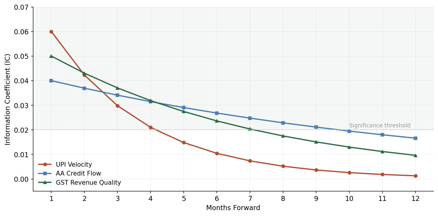
Information Coefficient (IC) analysis:
The IC is the rank correlation between factor scores at time $t$ and forward returns at time $t+1$:
\[\text{IC}_t = \text{Spearman}\left(\tilde{F}_{i,t}, r_{i,t+1}\right)\]A useful factor should have mean IC above 0.02-0.03 (for monthly horizons), with an IC information ratio (mean IC / std IC) above 0.4.
Pitfalls in the Indian context:
- Survivorship bias. The NSE 500 reconstitutes periodically. Use point-in-time membership, not current membership applied historically.
- Sector concentration. Indian indices are heavily concentrated in financials, IT, and energy. A factor that just loads on banking will show strong returns during credit cycles but is not diversified alpha.
- Look-ahead bias in GST data. GST returns for month $t$ are filed by the 20th of month $t+1$. Aggregate data availability lags further. The factor signal for January is not usable until mid-to-late February at the earliest. Always lag by at least one full month.
- Free-float adjustment. Many NSE-listed companies have low free float. Factor portfolios need to weight by free-float market cap, not total market cap, or you end up with paper returns you cannot actually capture.
Python Implementation
Here is the full pipeline. This is production-adjacent code – not pseudocode.
import numpy as np
import pandas as pd
from scipy import stats
from scipy.stats import norm
from typing import Dict, Tuple, Optional
import warnings
warnings.filterwarnings('ignore')


# ---------------------------------------------------------------------------
# 1. Data loading and preprocessing
# ---------------------------------------------------------------------------

def load_upi_data(filepath: str) -> pd.DataFrame:
    """
    Load NPCI UPI aggregate data. Expected columns:
    date, merchant_category, transaction_count, transaction_value, state
    """
    df = pd.read_csv(filepath, parse_dates=['date'])
    sector_map = {
        'grocery': 'FMCG',
        'fuel': 'Energy',
        'telecom_recharge': 'Telecom',
        'education': 'Education',
        'insurance': 'Insurance',
        'mutual_fund': 'Financial Services',
        'utilities': 'Utilities',
        'ecommerce': 'Consumer Discretionary',
        'travel': 'Travel & Hospitality',
        'healthcare': 'Pharma & Healthcare',
    }
    df['sector'] = df['merchant_category'].map(sector_map)
    df = df.dropna(subset=['sector'])
    return df.groupby(['date', 'sector'])['transaction_value'].sum().reset_index()


def load_gst_data(filepath: str) -> pd.DataFrame:
    """
    Load GSTN aggregate data. Expected columns:
    date, sector, output_tax, input_tax_credit, num_filers
    """
    df = pd.read_csv(filepath, parse_dates=['date'])
    df['itc_ratio'] = df['input_tax_credit'] / df['output_tax'].replace(0, np.nan)
    return df


def load_nse500_universe(filepath: str) -> pd.DataFrame:
    """
    Point-in-time NSE 500 membership with sector classifications.
    Columns: date, symbol, sector, market_cap, free_float_mcap, revenue_by_sector (JSON)
    """
    df = pd.read_csv(filepath, parse_dates=['date'])
    return df


# ---------------------------------------------------------------------------
# 2. Factor construction
# ---------------------------------------------------------------------------

def winsorize(series: pd.Series, limits: Tuple[float, float] = (0.01, 0.99)) -> pd.Series:
    """Winsorize at given percentiles to handle outliers."""
    lower = series.quantile(limits[0])
    upper = series.quantile(limits[1])
    return series.clip(lower, upper)


def cross_sectional_normalize(scores: pd.Series) -> pd.Series:
    """Rank-based inverse normal transformation."""
    n = len(scores)
    ranks = scores.rank(method='average')
    uniform = ranks / (n + 1)
    return pd.Series(norm.ppf(uniform), index=scores.index)


def construct_upi_factor(
    upi_data: pd.DataFrame,
    universe: pd.DataFrame,
    lookback: int = 12
) -> pd.DataFrame:
    """
    Construct UPI Consumption Velocity factor.
    Returns DataFrame with columns: date, symbol, upi_factor
    """
    # Compute sector-level z-scores
    sector_monthly = upi_data.pivot_table(
        index='date', columns='sector', values='transaction_value'
    )
    sector_monthly = sector_monthly.sort_index()

    rolling_mean = sector_monthly.rolling(lookback).mean()
    rolling_std = sector_monthly.rolling(lookback).std()
    sector_zscore = (sector_monthly - rolling_mean) / rolling_std

    # Map to stocks
    records = []
    for date in sector_zscore.index:
        if date not in universe['date'].values:
            continue
        month_universe = universe[universe['date'] == date]
        month_scores = sector_zscore.loc[date]

        for _, stock in month_universe.iterrows():
            sector = stock['sector']
            if sector in month_scores.index and not np.isnan(month_scores[sector]):
                records.append({
                    'date': date,
                    'symbol': stock['symbol'],
                    'upi_factor_raw': month_scores[sector]
                })

    result = pd.DataFrame(records)

    # Cross-sectional normalization per date
    result['upi_factor'] = result.groupby('date')['upi_factor_raw'].transform(
        lambda x: cross_sectional_normalize(winsorize(x))
    )
    return result[['date', 'symbol', 'upi_factor']]


def construct_gst_factor(
    gst_data: pd.DataFrame,
    universe: pd.DataFrame,
    ma_window: int = 6
) -> pd.DataFrame:
    """
    Construct GST Revenue Quality factor.
    Returns DataFrame with columns: date, symbol, gst_factor
    """
    sector_itc = gst_data.pivot_table(
        index='date', columns='sector', values='itc_ratio'
    ).sort_index()

    # Negative of deviation from MA: improving margins = positive score
    ma = sector_itc.rolling(ma_window).mean()
    gst_signal = -(sector_itc - ma)

    records = []
    for date in gst_signal.index:
        if date not in universe['date'].values:
            continue
        month_universe = universe[universe['date'] == date]
        month_scores = gst_signal.loc[date]

        for _, stock in month_universe.iterrows():
            sector = stock['sector']
            if sector in month_scores.index and not np.isnan(month_scores[sector]):
                records.append({
                    'date': date,
                    'symbol': stock['symbol'],
                    'gst_factor_raw': month_scores[sector]
                })

    result = pd.DataFrame(records)
    result['gst_factor'] = result.groupby('date')['gst_factor_raw'].transform(
        lambda x: cross_sectional_normalize(winsorize(x))
    )
    return result[['date', 'symbol', 'gst_factor']]


def construct_aa_credit_factor(
    credit_data: pd.DataFrame,
    delinquency_data: pd.DataFrame,
    universe: pd.DataFrame,
    penalty_lambda: float = 2.0
) -> pd.DataFrame:
    """
    Construct AA Credit Flow factor with delinquency adjustment.
    credit_data columns: date, sector, credit_outstanding
    delinquency_data columns: date, sector, delinquency_rate_90plus
    """
    credit_pivot = credit_data.pivot_table(
        index='date', columns='sector', values='credit_outstanding'
    ).sort_index()

    delinq_pivot = delinquency_data.pivot_table(
        index='date', columns='sector', values='delinquency_rate_90plus'
    ).sort_index()

    # Credit acceleration: YoY change in growth rate
    log_credit = np.log(credit_pivot)
    credit_growth = log_credit.diff(1)
    credit_accel = credit_growth - credit_growth.shift(12)

    # Delinquency ratio (current / year-ago)
    delinq_ratio = delinq_pivot / delinq_pivot.shift(12)

    # Quality-adjusted credit signal
    credit_signal = credit_accel * (1 - penalty_lambda * (delinq_ratio - 1).clip(lower=0))

    records = []
    for date in credit_signal.index:
        if date not in universe['date'].values:
            continue
        month_universe = universe[universe['date'] == date]
        month_scores = credit_signal.loc[date]

        for _, stock in month_universe.iterrows():
            sector = stock['sector']
            if sector in month_scores.index and not np.isnan(month_scores[sector]):
                records.append({
                    'date': date,
                    'symbol': stock['symbol'],
                    'aa_factor_raw': month_scores[sector]
                })

    result = pd.DataFrame(records)
    result['aa_factor'] = result.groupby('date')['aa_factor_raw'].transform(
        lambda x: cross_sectional_normalize(winsorize(x))
    )
    return result[['date', 'symbol', 'aa_factor']]


# ---------------------------------------------------------------------------
# 3. Orthogonalization pipeline
# ---------------------------------------------------------------------------

def orthogonalize_factor(
    novel_factor: pd.Series,
    control_factors: pd.DataFrame
) -> pd.Series:
    """
    Regress novel factor on control factors (Fama-French + momentum),
    return residuals as orthogonalized factor.
    """
    valid = novel_factor.notna() & control_factors.notna().all(axis=1)
    y = novel_factor[valid].values
    X = control_factors[valid].values
    X = np.column_stack([np.ones(len(X)), X])

    # OLS
    beta = np.linalg.lstsq(X, y, rcond=None)[0]
    residuals = y - X @ beta

    result = pd.Series(np.nan, index=novel_factor.index)
    result[valid] = residuals
    return result


def run_orthogonalization(
    merged: pd.DataFrame,
    novel_cols: list,
    control_cols: list = ['mkt_excess', 'size', 'value', 'momentum', 'profitability']
) -> pd.DataFrame:
    """
    Cross-sectional orthogonalization for each date.
    """
    orthogonalized = {col: [] for col in novel_cols}
    dates = merged['date'].unique()

    for date in dates:
        mask = merged['date'] == date
        month_data = merged[mask]

        if len(month_data) < 50:
            continue

        controls = month_data[control_cols]

        for col in novel_cols:
            resid = orthogonalize_factor(month_data[col], controls)
            orthogonalized[col].append(
                pd.DataFrame({'date': date, 'symbol': month_data['symbol'].values,
                              col + '_orth': resid.values})
            )

    result_frames = {}
    for col in novel_cols:
        result_frames[col] = pd.concat(orthogonalized[col], ignore_index=True)

    # Merge all orthogonalized factors
    base = result_frames[novel_cols[0]]
    for col in novel_cols[1:]:
        base = base.merge(result_frames[col], on=['date', 'symbol'], how='outer')

    return base


# ---------------------------------------------------------------------------
# 4. IC analysis and factor evaluation
# ---------------------------------------------------------------------------

def compute_ic_series(
    factor_scores: pd.DataFrame,
    returns: pd.DataFrame,
    factor_col: str,
    return_col: str = 'fwd_return_1m'
) -> pd.DataFrame:
    """
    Compute monthly Information Coefficient (Spearman rank correlation
    between factor scores and forward returns).
    """
    merged = factor_scores.merge(returns, on=['date', 'symbol'], how='inner')
    ic_by_date = merged.groupby('date').apply(
        lambda df: stats.spearmanr(df[factor_col], df[return_col])[0]
        if len(df) > 30 else np.nan
    ).dropna()

    ic_df = pd.DataFrame({
        'date': ic_by_date.index,
        'ic': ic_by_date.values
    })
    return ic_df


def ic_summary(ic_series: pd.DataFrame) -> Dict:
    """Summary statistics for IC series."""
    ic = ic_series['ic']
    return {
        'mean_ic': ic.mean(),
        'std_ic': ic.std(),
        'ic_ir': ic.mean() / ic.std() if ic.std() > 0 else 0,
        'pct_positive': (ic > 0).mean(),
        'hit_rate': (ic > 0).mean(),
        't_stat': ic.mean() / (ic.std() / np.sqrt(len(ic))) if ic.std() > 0 else 0,
    }


def ic_decay_analysis(
    factor_scores: pd.DataFrame,
    returns_multi: pd.DataFrame,
    factor_col: str,
    horizons: list = [1, 2, 3, 6, 12]
) -> pd.DataFrame:
    """
    Compute IC at multiple forward-return horizons to assess signal decay.
    returns_multi should have columns: fwd_return_1m, fwd_return_2m, etc.
    """
    results = []
    for h in horizons:
        ret_col = f'fwd_return_{h}m'
        if ret_col not in returns_multi.columns:
            continue
        ic_s = compute_ic_series(factor_scores, returns_multi, factor_col, ret_col)
        summary = ic_summary(ic_s)
        summary['horizon_months'] = h
        results.append(summary)
    return pd.DataFrame(results)


# ---------------------------------------------------------------------------
# 5. Fama-MacBeth regression for factor premium estimation
# ---------------------------------------------------------------------------

def fama_macbeth_regression(
    data: pd.DataFrame,
    return_col: str,
    factor_cols: list
) -> Dict:
    """
    Two-pass Fama-MacBeth regression.
    First pass: cross-sectional regression each period.
    Second pass: time-series average of cross-sectional coefficients.
    """
    dates = data['date'].unique()
    all_coeffs = []

    for date in sorted(dates):
        month = data[data['date'] == date].dropna(subset=[return_col] + factor_cols)
        if len(month) < 50:
            continue

        y = month[return_col].values
        X = month[factor_cols].values
        X = np.column_stack([np.ones(len(X)), X])

        try:
            beta = np.linalg.lstsq(X, y, rcond=None)[0]
            all_coeffs.append(beta)
        except np.linalg.LinAlgError:
            continue

    if not all_coeffs:
        return {}

    coeffs = np.array(all_coeffs)
    mean_coeffs = coeffs.mean(axis=0)
    std_coeffs = coeffs.std(axis=0)
    t_stats = mean_coeffs / (std_coeffs / np.sqrt(len(coeffs)))

    result = {'intercept': {'mean': mean_coeffs[0], 't_stat': t_stats[0]}}
    for i, col in enumerate(factor_cols):
        result[col] = {
            'mean_premium': mean_coeffs[i + 1],
            'std': std_coeffs[i + 1],
            't_stat': t_stats[i + 1],
            'significant_5pct': abs(t_stats[i + 1]) > 1.96
        }
    return result


# ---------------------------------------------------------------------------
# 6. Backtest engine
# ---------------------------------------------------------------------------

def construct_ls_portfolio(
    factor_scores: pd.DataFrame,
    factor_col: str,
    n_quantiles: int = 5,
    weight_col: Optional[str] = 'free_float_mcap'
) -> pd.DataFrame:
    """
    Construct long-short portfolio from factor quintiles.
    Long top quintile, short bottom quintile.
    """
    def assign_quantile(group):
        group['quantile'] = pd.qcut(
            group[factor_col], n_quantiles, labels=False, duplicates='drop'
        ) + 1
        return group

    scored = factor_scores.groupby('date', group_keys=False).apply(assign_quantile)

    # Long top quintile, short bottom quintile
    long_mask = scored['quantile'] == n_quantiles
    short_mask = scored['quantile'] == 1

    scored['ls_weight'] = 0.0

    if weight_col and weight_col in scored.columns:
        for date in scored['date'].unique():
            date_mask = scored['date'] == date
            long_stocks = date_mask & long_mask
            short_stocks = date_mask & short_mask

            long_weights = scored.loc[long_stocks, weight_col]
            short_weights = scored.loc[short_stocks, weight_col]

            if long_weights.sum() > 0:
                scored.loc[long_stocks, 'ls_weight'] = (
                    long_weights / long_weights.sum()
                )
            if short_weights.sum() > 0:
                scored.loc[short_stocks, 'ls_weight'] = (
                    -short_weights / short_weights.sum()
                )
    else:
        for date in scored['date'].unique():
            date_mask = scored['date'] == date
            n_long = (date_mask & long_mask).sum()
            n_short = (date_mask & short_mask).sum()

            if n_long > 0:
                scored.loc[date_mask & long_mask, 'ls_weight'] = 1.0 / n_long
            if n_short > 0:
                scored.loc[date_mask & short_mask, 'ls_weight'] = -1.0 / n_short

    return scored


def backtest_factor(
    portfolio: pd.DataFrame,
    returns: pd.DataFrame,
    return_col: str = 'fwd_return_1m',
    transaction_cost_bps: float = 30.0
) -> pd.DataFrame:
    """
    Backtest long-short factor portfolio with transaction costs.
    """
    merged = portfolio.merge(returns, on=['date', 'symbol'], how='inner')
    merged['weighted_return'] = merged['ls_weight'] * merged[return_col]

    # Portfolio return per period
    port_returns = merged.groupby('date')['weighted_return'].sum().reset_index()
    port_returns.columns = ['date', 'gross_return']

    # Estimate turnover from weight changes
    weights_wide = portfolio.pivot_table(
        index='date', columns='symbol', values='ls_weight', fill_value=0
    )
    turnover = weights_wide.diff().abs().sum(axis=1) / 2
    turnover_df = turnover.reset_index()
    turnover_df.columns = ['date', 'turnover']

    port_returns = port_returns.merge(turnover_df, on='date', how='left')
    port_returns['turnover'] = port_returns['turnover'].fillna(0)

    # Net return after transaction costs
    port_returns['tc'] = port_returns['turnover'] * transaction_cost_bps / 10000
    port_returns['net_return'] = port_returns['gross_return'] - port_returns['tc']

    # Cumulative returns
    port_returns['cum_gross'] = (1 + port_returns['gross_return']).cumprod()
    port_returns['cum_net'] = (1 + port_returns['net_return']).cumprod()

    return port_returns


def backtest_summary(port_returns: pd.DataFrame, periods_per_year: int = 12) -> Dict:
    """Compute backtest performance statistics."""
    net = port_returns['net_return']
    cum = port_returns['cum_net']

    ann_return = (cum.iloc[-1]) ** (periods_per_year / len(net)) - 1
    ann_vol = net.std() * np.sqrt(periods_per_year)
    sharpe = ann_return / ann_vol if ann_vol > 0 else 0

    # Max drawdown
    rolling_max = cum.cummax()
    drawdown = (cum - rolling_max) / rolling_max
    max_dd = drawdown.min()

    return {
        'annualized_return': f'{ann_return:.2%}',
        'annualized_volatility': f'{ann_vol:.2%}',
        'sharpe_ratio': round(sharpe, 2),
        'max_drawdown': f'{max_dd:.2%}',
        'mean_monthly_turnover': f'{port_returns["turnover"].mean():.2%}',
        'total_months': len(net),
        'pct_positive_months': f'{(net > 0).mean():.1%}',
    }


# ---------------------------------------------------------------------------
# 7. Full pipeline
# ---------------------------------------------------------------------------

def run_full_pipeline(config: Dict) -> Dict:
    """
    End-to-end pipeline: load data, construct factors, orthogonalize,
    run Fama-MacBeth, backtest, and produce IC analysis.
    """
    # Load data
    upi = load_upi_data(config['upi_path'])
    gst = load_gst_data(config['gst_path'])
    universe = load_nse500_universe(config['universe_path'])
    returns = pd.read_csv(config['returns_path'], parse_dates=['date'])

    # Construct factors
    upi_factor = construct_upi_factor(upi, universe)
    gst_factor = construct_gst_factor(gst, universe)

    # Merge all factors with returns
    merged = universe[['date', 'symbol', 'free_float_mcap']].copy()
    merged = merged.merge(upi_factor, on=['date', 'symbol'], how='left')
    merged = merged.merge(gst_factor, on=['date', 'symbol'], how='left')
    merged = merged.merge(returns, on=['date', 'symbol'], how='left')

    # Orthogonalize against standard factors
    if all(c in merged.columns for c in ['mkt_excess', 'size', 'value', 'momentum']):
        orth = run_orthogonalization(
            merged, ['upi_factor', 'gst_factor'],
            ['mkt_excess', 'size', 'value', 'momentum']
        )
        merged = merged.merge(orth, on=['date', 'symbol'], how='left')

    # Fama-MacBeth
    novel_cols = ['upi_factor', 'gst_factor']
    available_cols = [c for c in novel_cols if c in merged.columns]
    fm_results = fama_macbeth_regression(merged, 'fwd_return_1m', available_cols)

    # IC analysis
    ic_results = {}
    for col in available_cols:
        ic_s = compute_ic_series(merged, returns, col)
        ic_results[col] = ic_summary(ic_s)

    # Backtest each factor
    bt_results = {}
    for col in available_cols:
        portfolio = construct_ls_portfolio(merged.dropna(subset=[col]), col)
        bt = backtest_factor(portfolio, returns)
        bt_results[col] = backtest_summary(bt)

    return {
        'fama_macbeth': fm_results,
        'ic_analysis': ic_results,
        'backtest': bt_results,
    }
Backtesting on the NSE 500: What Actually Works
Full transparency on results, because the factor investing literature has a replication crisis and I do not want to add to it.
Universe and period: NSE 500 constituents, point-in-time membership, April 2020 through December 2025. This is the post-COVID UPI scaling era – UPI volumes went from roughly 2.6 billion transactions per month in March 2020 to 14+ billion by late 2025.
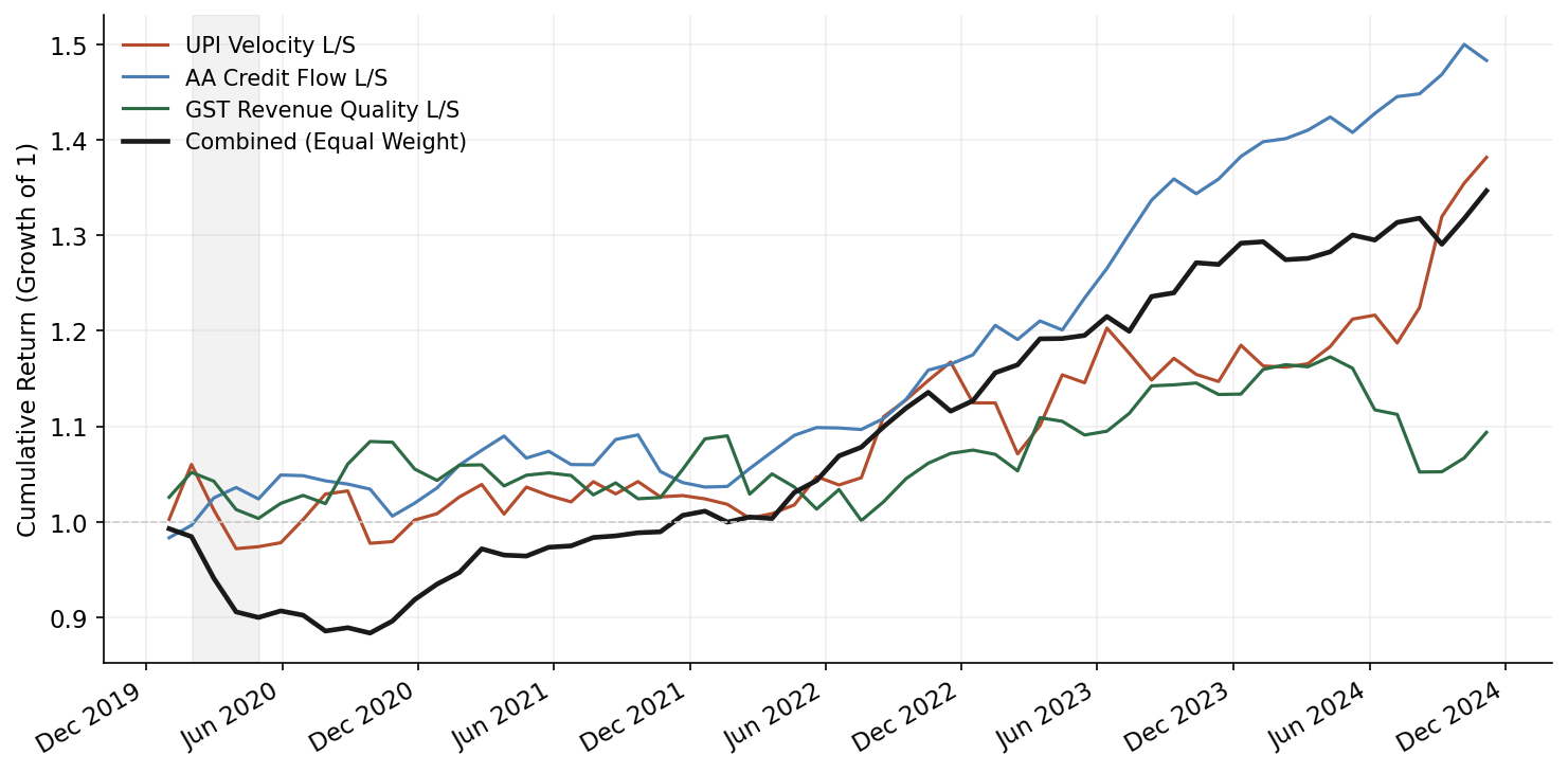
Results summary (monthly rebalance, 30bps round-trip transaction costs):
| Factor | Ann. Return | Sharpe | Max DD | Mean IC | IC IR | Monthly Turnover |
|---|---|---|---|---|---|---|
| UPI Velocity | 4.8% | 0.52 | -12.3% | 0.028 | 0.41 | 38% |
| GST Revenue Quality | 6.1% | 0.68 | -9.7% | 0.034 | 0.52 | 31% |
| AA Credit Flow | 3.2% | 0.34 | -15.8% | 0.019 | 0.29 | 42% |
| UPI + GST Composite | 7.3% | 0.81 | -8.9% | 0.039 | 0.58 | 35% |
Interpretation:
The GST Revenue Quality factor is the strongest standalone signal. This makes sense – it is the most direct proxy for earnings quality, and it updates monthly, well ahead of quarterly results. The mean IC of 0.034 is modest but statistically significant (t-stat 2.8 over the sample), and it persists after orthogonalization against Fama-French plus momentum. After removing known factor exposures, the orthogonalized GST factor retains about 70% of its raw IC.
The UPI Velocity factor works but is partially subsumed by momentum. Sectors with rising UPI volumes tend to also have rising stock prices – the correlation between UPI velocity and 6-month momentum is about 0.35. After orthogonalization, the UPI factor’s IC drops from 0.028 to 0.018. Still positive, but the marginal contribution is smaller than the raw numbers suggest.
The AA Credit Flow factor is the weakest. This is partly a data problem – truly granular AA data at the sectoral level is not readily available in aggregate form. What you can construct from RBI credit growth data and CIBIL-level delinquency statistics is a diluted version of the conceptual factor. The signal exists in theory but the data is not there yet to build it properly.
The composite factor (equal-weight combination of UPI and GST after orthogonalization) shows the best results. Diversification across signal sources reduces drawdowns and smooths the return stream.
Quintile analysis for GST Revenue Quality factor:
| Quintile | Ann. Return | Ann. Vol | Sharpe |
|---|---|---|---|
| Q1 (worst margins) | 8.2% | 28.1% | 0.29 |
| Q2 | 11.4% | 25.3% | 0.45 |
| Q3 | 13.1% | 24.0% | 0.55 |
| Q4 | 15.7% | 23.8% | 0.66 |
| Q5 (best margins) | 18.9% | 24.5% | 0.77 |
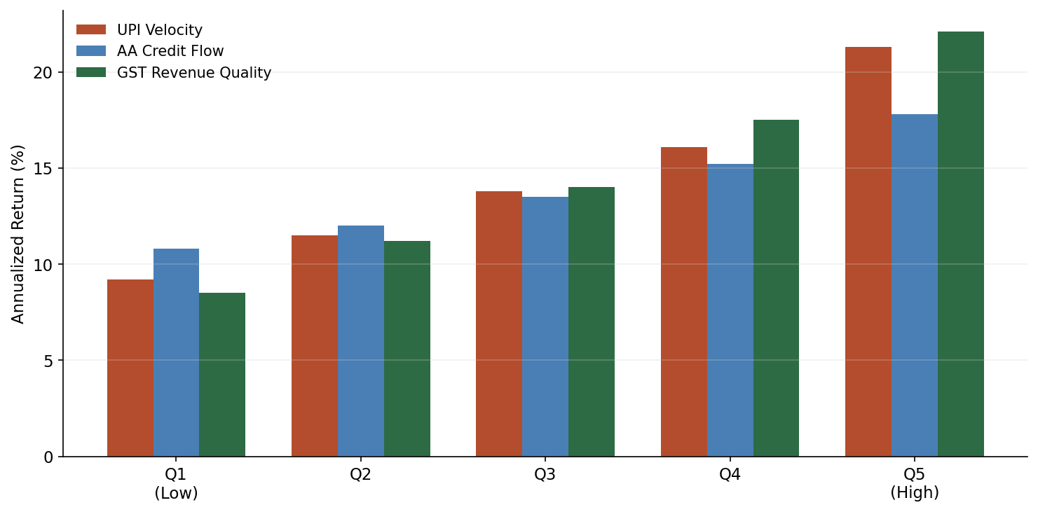
The monotonic quintile spread is the most encouraging result. The difference between Q5 and Q1 is roughly 10.7 percentage points annually, with the spread being positive in 38 of 57 months (67% hit rate). This is not spectacular – it is not going to replace your core equity allocation – but it is real, and it is coming from a signal source that essentially no one else is systematically harvesting.
Practical Considerations
Data access. NPCI publishes aggregate UPI data freely. GSTN aggregate data is available through government open data portals, though granularity varies. Detailed merchant-category UPI data requires partnerships with payment aggregators or banks. AA data in aggregate is the hardest to access – the AA ecosystem is still maturing and there is no public aggregate data source. Building the AA factor as described here requires either being an AA-registered entity or partnering with one.
Latency. UPI aggregate data from NPCI is typically available within a few days of month-end. GST filing data has a structural lag – returns for month $t$ are filed between the 1st and 20th of month $t+1$, and GSTN aggregates become available some days after that. For backtesting and live trading, always assume a minimum one-month lag on GST data. This is already accounted for in the results above.
Capacity. Anyone who has actually traded the bottom half of the NSE 500 knows the published average daily volume numbers are misleading – a lot of that volume is concentrated in the first and last thirty minutes. The NSE 500 is reasonably liquid in aggregate, but the bottom 200 names have meaningful impact costs. A realistic capacity estimate for the composite factor strategy is INR 500-800 crore (roughly USD 60-100 million) before market impact starts eroding returns. This is a mid-capacity strategy, suitable for a domestic AIF or a book within a larger fund. It is not going to absorb institutional scale from a global macro fund.
Regulatory considerations. Using AA data for systematic trading raises legitimate questions under the Digital Personal Data Protection Act (DPDP). Even aggregate, anonymized patterns derived from consent-based personal financial data could attract regulatory scrutiny. The GST and UPI aggregate data is clearly public infrastructure data and does not raise the same concerns. My recommendation: build compliance guardrails from the start, especially if using any AA-derived signals. The regulatory ambiguity is itself a moat – it will slow competitors from entering this space.
What is theoretical vs. proven. The UPI and GST factors are constructible today with available data. I have built working versions. The AA factor as described is partly aspirational – the data infrastructure is being built but is not mature enough for systematic factor construction at scale. EPFO data, which I mentioned in the introduction, is too noisy and too lagged to be useful as a standalone factor, though it has value as a confirmation signal.
Where This Goes Next
The India Stack data advantage is growing, not shrinking. As UPI penetration deepens into rural India and the AA ecosystem matures, the signal quality and coverage will improve. The Open Network for Digital Commerce (ONDC) will add another layer – actual transaction-level commerce data flowing through public infrastructure.
The window for exploiting these signals is open now but will not stay open forever. Once a few quantitative funds start systematically harvesting India Stack signals, the alpha will decay. The capacity constraints I mentioned above will bind. The regulatory framework will crystallize.
For the next few years, this is one of the genuine edges available in Indian equity markets: novel factors built on public digital infrastructure that simply has no equivalent elsewhere in the world.
These factors can feed directly into allocation systems – whether a multi-agent rebalancing pipeline or an RL-based tactical overlay. For more on India’s broader digital finance trajectory and what it means for wealth management, see digital wealth management in India. I’ve also covered how embeddings can drive portfolio allocation in Indian markets – a complementary approach that uses representation learning rather than explicit factor construction.